Start with the exam
What you need to be able to do
This section is a mixed archive, not a single current-syllabus topic. Its early questions contain transferable experimental skills: uncertainty, zero corrections, dimensional analysis and graph models. Later material includes historical options such as specialised optics, capacitors, medical imaging, particle classifications and cosmology. Use each bank compatibility label before deciding what to revise for your examination. The lesson prioritises experimental reasoning that transfers to current questions; it does not imply that all archived option content is required.
Spend 3 minutes reading the overview and diagram, 7 minutes learning the question patterns, 5 minutes writing out the worked example, and 5 minutes on a bank question or recall check. Take longer when you need to; the full bank is here for later practice.
This collection contains content outside the current course, or a mixture of current and legacy skills. Use the compatibility note for each original question to decide which parts to practise for your exam.
Recognise → set up → write
How the questions are set
Correct measurements and propagate uncertainty
Recognise it: A zero reading, density estimate, measured difference or power of a quantity appears.
- Correct the measured value for the instrument offset with its sign. If an empty instrument reads −0.02 mm, add 0.02 mm to later readings before using them.
- For sums or differences, combine absolute uncertainties using the stated school/exam convention; for products and quotients, combine fractional uncertainties. A power n multiplies fractional uncertainty by |n| in the usual small-uncertainty estimate.
- For a claim such as “this sample is pure”, compare the result’s plausible uncertainty interval with the reference value. Agreement means consistency within uncertainty, not proof that the model or purity claim is certainly true.
Since volume is proportional to d³, its fractional uncertainty is approximately three times the fractional diameter uncertainty.
Subtracting two nearly equal measurements can leave a small result with a large relative uncertainty.
Linearise a model and interpret the fit
Recognise it: A supplied equation, transformed axes, best-fit line or maximum/minimum gradient is given.
- Rearrange the supplied model into y = mx + c using the actual plotted variables. Identify what physical combination the gradient represents and what the intercept should be.
- Use well-separated points on the best-fit line, preserving axis scale factors. For uncertainty, draw or evaluate the steepest and shallowest acceptable lines using the error bars and the method requested.
- A straight-looking trend does not prove proportionality: proportionality also requires consistency with a zero intercept. Compare residual patterns, uncertainty ranges and the expected intercept before accepting the model.
The fitted line tests the model only if its gradient, intercept and uncertainty are interpreted in terms of the rearranged equation.
Two chosen data points do not substitute for a best-fit analysis across the complete data set.
Transfer the mathematics without importing obsolete scope
Recognise it: An archived option gives attenuation, an exponential decay, a new coefficient or a specialised device.
- Read the compatibility note first. Separate the current transferable calculation from the historical physical background; the presence of a familiar equation does not make every subpart current.
- For a supplied exponential model, normalise the measured quantity, take logarithms if needed and identify the coefficient from the transformed gradient. Check dimensions so an exponential argument is dimensionless.
- For explanations about a specialised instrument, distinguish what is provided in the question from extra knowledge required by the historical option. Use this as extension work only after the targeted current material is secure.
Using the supplied model, ln(I/I₀) = −μx, so the gradient of the transformed graph is −μ and μ has units of inverse length.
An archived capacitor, cosmology or imaging question should not be treated as evidence that all its specialist content belongs to the current course.
Write it before you reveal it
A worked exam-style example
Original teaching example, created for this lesson.
A sphere has corrected diameter (10.0 ± 0.1) mm and mass (4.0 ± 0.1) g. Estimate its density and percentage uncertainty using additive fractional uncertainties.
Reveal the worked solution
- Volume V = πd³/6 = π × 1.00³/6 = 0.5236 cm³, since 10.0 mm = 1.00 cm.
- Density is 4.0/0.5236 = 7.64 g cm⁻³. Diameter fractional uncertainty is 1%, giving volume uncertainty 3%.
- Mass fractional uncertainty is 0.1/4.0 = 2.5%. Add for density: 2.5% + 3.0% = 5.5%, equivalent to approximately 0.42 g cm⁻³.
Answer: Density ≈ (7.6 ± 0.4) g cm⁻³; percentage uncertainty ≈ 5.5%.
Check: The uncertainty is dominated jointly by mass and cubed diameter; reporting many decimal places would imply unjustified precision.
From your own collection
Apply it to past-paper questions
These questions anchor the patterns above. Attempt one without the answer, then compare your setup and conclusion with the reasoning. The linked reader contains the source answer and the question-specific syllabus review.
Question 1323
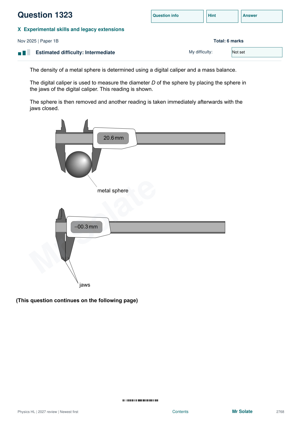
Corrects a negative zero reading and propagates a cubic diameter uncertainty.
Compatibility: All parts practise current Physics HL concepts and experimental skills. The stated model and supplied relations should be used.
View the original question
Original page images preserve the equations and diagrams. Write your response before revealing the reasoning.
Reveal the revision reasoning
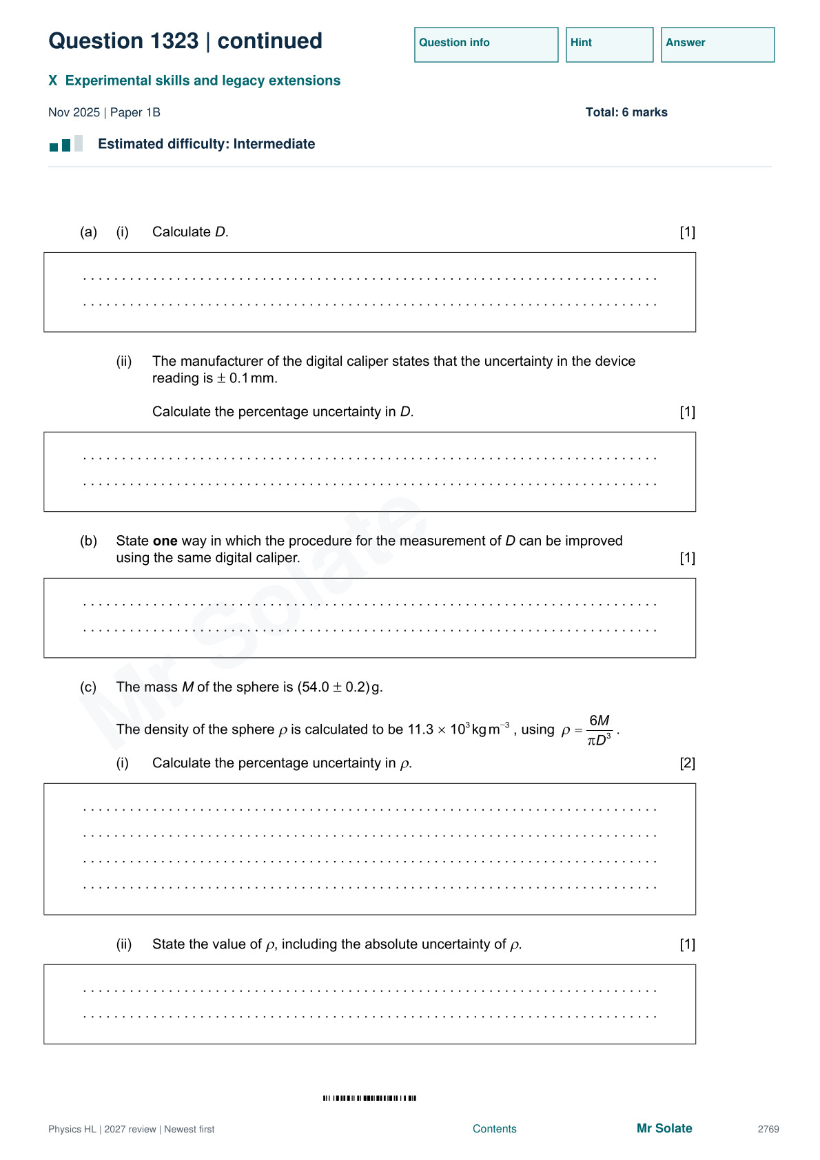
The corrected diameter is 20.6-(-0.3)=20.9mm. Combining the two0.1mm reading uncertainties gives 0.2mm, about 0.96%. Repeat in several orientations to check sphericity and reduce random scatter.
For rho=6M/(pi D^3), add fractional mass uncertainty and three times the fractional diameter uncertainty. This gives about 3.2%, so the density is approximately(11.3±0.4)×10^3kg/m^3.
Editorial revision reasoning. Check the original answer for its marking detail.
Question 1362
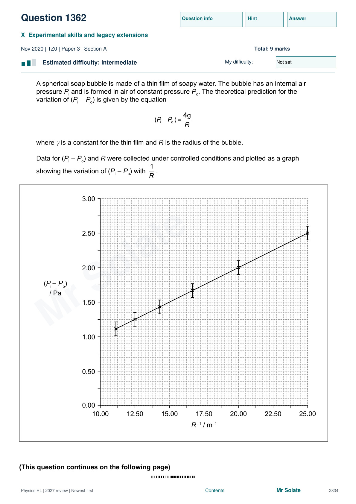
Requires reading a transformed graph, dimensional analysis and a worst-fit uncertainty estimate.
Compatibility: All parts are current experimental/data-analysis skills using the supplied bubble model; prior surface-tension theory is not required.
View the original question
Original page images preserve the equations and diagrams. Write your response before revealing the reasoning.
Reveal the revision reasoning
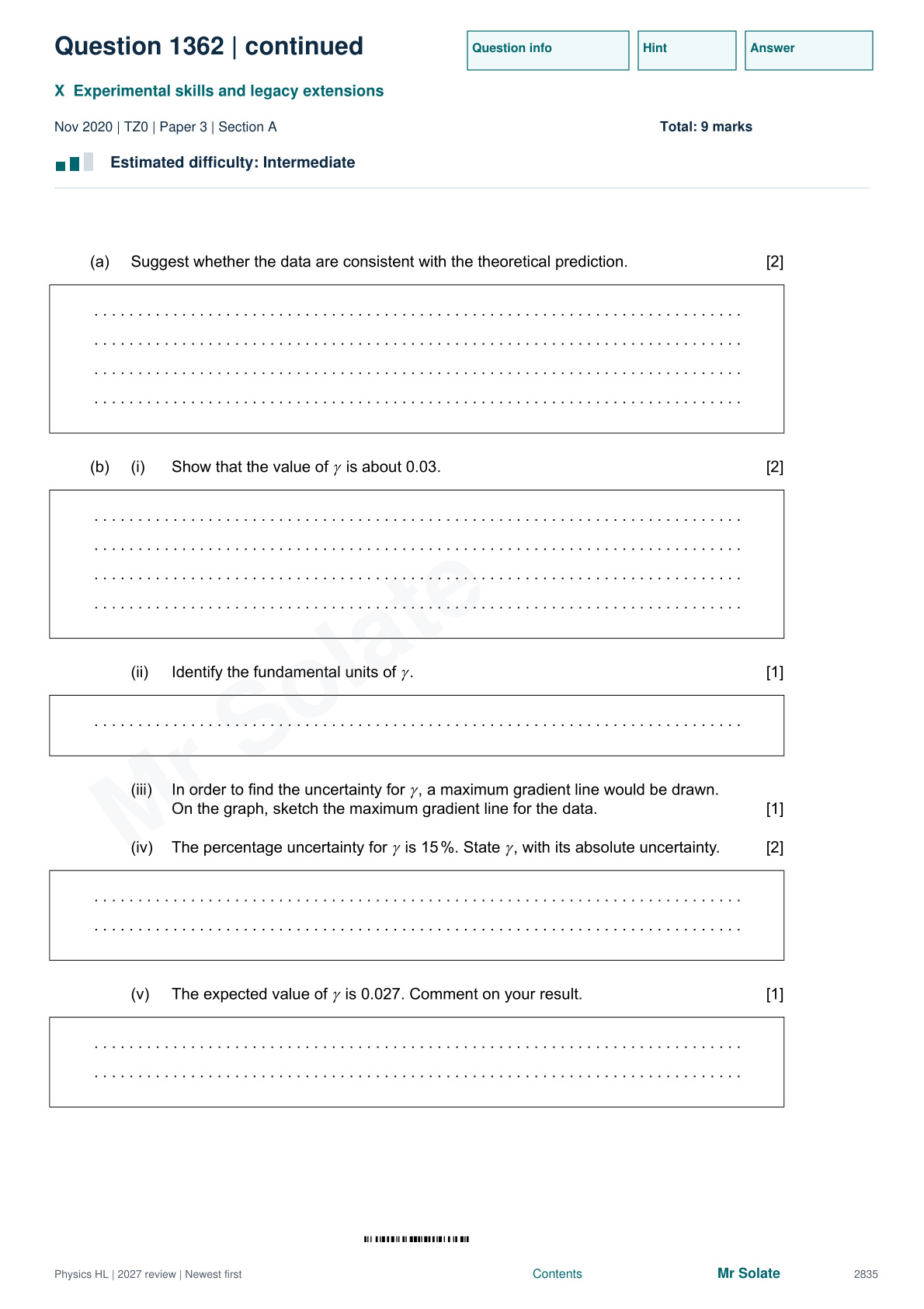
Assess whether a straight line through the origin fits the error bars, then divide a large-triangle gradient by four.
Gamma has units Pa m, equivalent to kg s^-2; draw the steepest line still compatible with the data.
Convert 15% to an absolute uncertainty and check whether 0.027 lies inside the result’s interval.
Editorial revision reasoning. Check the original answer for its marking detail.
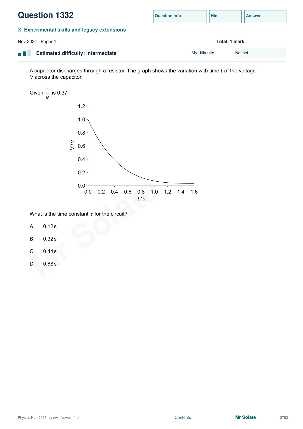
Question 1332
Reads an exponential time constant at 37% of initial voltage.
Compatibility: RC capacitor discharge is legacy content outside current B.5. Use the additional exponential law V=V₀e^(−t/RC).
View the original question
Original page images preserve the equations and diagrams. Write your response before revealing the reasoning.
Reveal the revision reasoning
The starting voltage is 1.0 V. Reading the time at 0.37 V gives approximately 0.44 s.
Editorial revision reasoning. Check the original answer for its marking detail.
All 113 questions in this topic
Close your notes first
Can you retrieve the method?
1. Does agreement within uncertainty prove a model correct?
Check answer 1
No; it shows the measurement is consistent with the model at that precision.
2. What extra condition distinguishes proportionality from a general straight line?
Check answer 2
An intercept consistent with zero.
3. Does an archived option question automatically belong to the current course?
Check answer 3
No; use its compatibility note and isolate transferable parts.
Before you move on
- Prioritise current-compatible experimental questions before specialist legacy extensions.
- Finish every uncertainty answer with a physical conclusion tied to the uncertainty range.
Your revision note
Record one missed cue, one corrected step and one question to retry. Saved only in this browser.